2 minutes
Benchmark Confidence Interval Part 2: Comparison
Benchmark data generally isn’t interesting in isolation; once we have one data set, we usually gather a second set of data against which the first is compared. Reporting the second result as a percentage of the first result isn’t sufficient if we’re rigorous and report results with confidence intervals; we need a more nuanced approach.
Let’s suppose we run a benchmark 5 times and record the results, then fix a performance bug and gather a second set of data to measure the improvement. The best intuition about performance gains is given by scores and confidence intervals that are normalized using our baseline geomean score:
All normalization is done using the same baseline, even the bug fix confidence interval. One
can work out the normalized confidence intervals for a baseline score of 100 +/- 1 and a
second score of 2 +/- 1 to see why this must be so.
Now, let’s visualize (using a LibreOffice Calc chart with custom Y error bars):
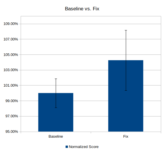
Woops! The confidence intervals overlap; something’s wrong here. We can’t be confident our performance optimization will reliably improve the performance of the benchmark unless 95% of our new results fall outside 95% of our old results. Something is dragging down our score and we cannot confidently reject our null hypothesis.
The root causes for such negative results are rich and diverse, but for illustrative purposes, let’s suppose we missed an edge case in our performance optimization that interacted badly with a power management algorithm. Our intrepid product team has fixed this issue, and now we have:
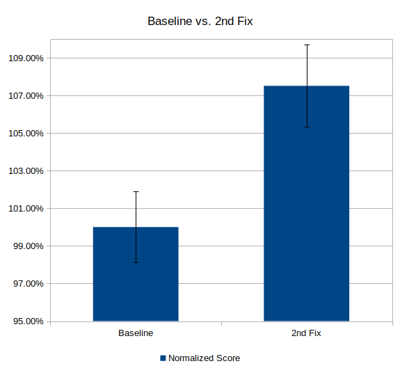
Much better; we can confidently reject the null hypothesis and assert that our latest fix has indeed improved performance of this benchmark.
Many thanks to Felix Degrood for his help in developing my understanding of these concepts and tools